Python training UGA 2017
A training to acquire strong basis in Python to use it efficiently
Pierre Augier (LEGI), Cyrille Bonamy (LEGI), Eric Maldonado (Irstea), Franck Thollard (ISTerre), Oliver Henriot (GRICAD), Christophe Picard (LJK), Loïc Huder (ISTerre)
Python scientific ecosystem
A short introduction to Matplotlib (gallery)
The default library to plot data is matplotlib. It allows one the creation of graphs that are ready for publications with the same functionality than Matlab.
# these ipython commands load special backend for notebooks
# (do not use "notebook" outside jupyter)
# %matplotlib notebook
# for jupyter-lab:
# %matplotlib ipympl
%matplotlib inline
When running code using matplotlib, it is highly recommended to start ipython with the option --matplotlib (or to use the magic ipython command %matplotlib).
Basic plotting with plot
import numpy as np
import matplotlib.pyplot as plt
y = np.random.random(5)
print(y)
[0.10778744 0.2393634 0.28269046 0.10192736 0.54835694]
lines = plt.plot(y)

plt.show()
Giving specific coordinates
x = np.linspace(0, 2, 20)
y = x**2

plt.figure()
plt.plot(x, y)
[<matplotlib.lines.Line2D at 0x7fab75857910>]

Figures and subplots
We can associate the figure and the system of axes to objects. These objects will allow us to add labels, modify the axis or save the figure.
The Figure object (in fig) handles the whole figure while the AxesSubplot object (in ax) handles the axes' system (called a subplot in matplotlib).
fig, ax = plt.subplots()
# Old syntax:
# fig = plt.figure()
# ax = fig.add_subplot(111)
ax.plot(x, y)

# Example: Change x and y labels
ax.set_xlabel('$Re$')
ax.set_ylabel('$\Pi / \epsilon$')
Text(0, 0.5, '$\\Pi / \\epsilon$')

Multiple subplots
fig, subplots = plt.subplots(nrows=2, ncols=1)
ax1, ax2 = subplots
X = np.arange(0, 2*np.pi, 0.1)
ax1.plot(X, np.cos(2*X), color="red")
ax2.plot(X, np.sin(2*X), color="magenta")
ax2.set_xlabel('Angle (rad)')
Text(0.5, 0, 'Angle (rad)')

fig, ax = plt.subplots()
res = ax.plot(x, y, color="red", linestyle='dashed', linewidth=3, marker='o',
        markerfacecolor='blue', markersize=5)

We can also recover the plotted matplotlib object to get info on it.
line_object = res[0]
print(type(line_object))
print('Color of the line is', line_object.get_color())
print('X data of the plot:', line_object.get_xdata())
<class 'matplotlib.lines.Line2D'>
Color of the line is red
X data of the plot: [0.         0.10526316 0.21052632 0.31578947 0.42105263 0.52631579
 0.63157895 0.73684211 0.84210526 0.94736842 1.05263158 1.15789474
 1.26315789 1.36842105 1.47368421 1.57894737 1.68421053 1.78947368
 1.89473684 2.        ]
Titles, labels and legends
Titles can be added to figures and subplots. Labels can be added when plotting to generate a legend afterwards.
x = np.arange(0, 2, 0.01)

fig, ax = plt.subplots()
ax.plot(x, x**2, label='$x^2$')
ax.plot(x, x**3, label='$x^3$')
ax.plot(x, np.exp(x) - 1, label='$e^{x} - 1$')
ax.set_title('Upscaling')
ax.legend()
fig.suptitle('FIGURE', fontweight='bold')
Text(0.5, 0.98, 'FIGURE')

Note that legends are attached to subplots. Note also the difference between the subplot title and the title of the figure.
Anatomy of a Matplotlib figure
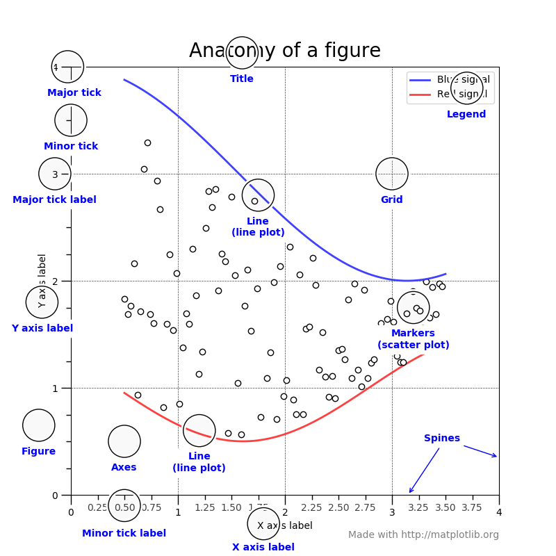
For consistent figure changes, define your own stylesheets that are basically a list of parameters to tune the aspect of the figure elements. See https://matplotlib.org/tutorials/introductory/customizing.html for more info.
2D plots
There are two main methods:
imshow: for square grids. X, Y are the center of pixels and (0,0) is top-left by default.pcolormesh(orpcolor): for non-regular rectangular grids. X, Y are the corners of pixels and (0,0) is bottom-left by default.
noise = np.random.random((10,10))

f, subplots = plt.subplots(1, 2)
subplots[0].imshow(noise)
subplots[1].pcolormesh(noise)
<matplotlib.collections.QuadMesh at 0x7fab754f0cd0>

We can also add a colorbar and adjust the colormap.
plt.figure()
plt.imshow(noise, cmap='Greys_r')
plt.colorbar()
<matplotlib.colorbar.Colorbar at 0x7fab754530d0>

Generate meshes with meshgrid
When in need of plotting a 2D function, it is useful to use meshgrid that wil generate a 2D mesh from the values of abscissas and ordinates
x = np.linspace(-2*np.pi, 2*np.pi, 200)
y = x

meshX, meshY = np.meshgrid(x, y)
Z = np.cos(2*meshX) + np.cos(4*meshY)

plt.figure()
plt.pcolormesh(meshX, meshY, Z, cmap='RdBu')
plt.colorbar()
<matplotlib.colorbar.Colorbar at 0x7fab753f2710>

Choosing colormaps
When doing such colorplots, it is easy to lose the interesting features by setting a colormap that is not adapted to the data. As a rule of thumb:
- use sequential colormaps for data varying continously from a value to another (ex: x^2 for positive values)
- use divergent colormaps for data varying around a mean value (ex: cos(x))
Also, when producing scientific figures, think about how will your plot will look like to colorblind people or in greyscales (as it can happen in printed articles...).
See the interesting discussion on matplotlib website: https://matplotlib.org/users/colormaps.html.
f, subplots = plt.subplots(1, 2)
plot1 = subplots[0].imshow(Z, cmap=plt.cm.jet)
f.colorbar(plot1, ax=subplots[0])
plot2 = subplots[1].imshow(Z, cmap=plt.cm.RdBu)
f.colorbar(plot2, ax=subplots[1])
<matplotlib.colorbar.Colorbar at 0x7fab7408bfd0>

# 3D example
from mpl_toolkits.mplot3d import Axes3D

fig = plt.figure()
ax = fig.add_subplot(111, projection='3d')

ax.plot_surface(meshX, meshY, np.exp(-(meshX**2+meshY**2)), cmap='viridis')
<mpl_toolkits.mplot3d.art3d.Poly3DCollection at 0x7fab6f7682d0>

Do it yourself:
The pratical work below is mostly manipulation of an image (2D data). See TP5 for manipulation/plotting of 1D data.
With miscellaneous routines of scipy, we can get an example image:
import scipy.misc
raccoon = np.array(scipy.misc.face())
Write a script to print shape and dtype the raccoon image. Next plot the image using matplotlib.
print("shape of raccoon = ", raccoon.shape)
print("dtype of raccoon = ", raccoon.dtype)
shape of raccoon =  (768, 1024, 3)
dtype of raccoon =  uint8
plt.imshow(raccoon)
<matplotlib.image.AxesImage at 0x7fab6eef98d0>

Write a script to generate a border around the raccoon image (for example a 20 pixel size black border; black color code is 0 0 0)
Do it again without losing pixels and generate then a raccoon1 array/image
- Mask the face of the raccoon with a grey circle (centered of radius 240 at location 690 260 of the raccoon1 image; grey color code is for example (120 120 120))
- Mask the face of the raccon with a grey square by using NumPy broadcast capabilities (height and width 480 and same center as before)
We propose to smooth the image : the value of a pixel of the smoothed image is the the average of the values of its neighborhood (ie the 8 neighbors + itself).
Solution 0
Write a script to generate a border around the raccoon image (for example a 20 pixel size black border; black color code is 0 0 0)
raccoon[0:20, :, :] = 0
raccoon[-20:-1, :, :] = 0
raccoon[:, 0:20, :] = 0
raccoon[:, -20:-1, :] = 0
plt.imshow(raccoon)
<matplotlib.image.AxesImage at 0x7fab6ef34750>

Solution 1
Do it again without losing pixels and generate then a raccoon1 array/image
raccoon = np.array(scipy.misc.face())
print("shape of raccoon = ", raccoon.shape)
n0, n1, n2 = raccoon.shape
raccoon1 = np.zeros((n0+40, n1+40, n2), dtype = np.uint8)
raccoon1[20:20+n0, 20:20+n1, :] = raccoon[:,:,:]
print("shape of raccoon1 = ", raccoon1.shape)
plt.imshow(raccoon1)
shape of raccoon =  (768, 1024, 3)
shape of raccoon1 =  (808, 1064, 3)
<matplotlib.image.AxesImage at 0x7fab6eeedf10>

Solution 2.A
Mask the face of the raccoon with a grey circle (centered of radius 240 at location 690 260 of the raccoon1 image; grey color code is for example (120 120 120))
raccoon2A = raccoon1.copy()

def anonymise_raccoon1_loop():
    x_center = 260
    y_center = 690
    radius = 240
    x_max, y_max, z = raccoon2A.shape
    for i in range(x_max):
        for j in range(y_max):
            if ((j - y_center)**2 + (i-x_center)**2) <= radius**2:
                raccoon2A[i, j, :] = 120

%timeit anonymise_raccoon1_loop()
plt.imshow(raccoon2A)
610 ms ± 15.6 ms per loop (mean ± std. dev. of 7 runs, 1 loop each)
<matplotlib.image.AxesImage at 0x7fab6eeacad0>

Solution 2.A.2 (vectorization and broadcasting)¶¶
raccoon2B = raccoon1.copy()

def annonymize_raccon1_vect():

    """
    i) build two matrix distance
    ii) build a condition (ie distance < radius)
    iii) affectation of point within tha satisfy the condition to 120

    for i) we use broadcasting (see e.g. https://i.stack.imgur.com/JcKv1.png)
    """

    x_center = 260
    y_center = 690
    radius = 240
    nb_lines, nb_cols, z = raccoon2B.shape
    x, y = np.ogrid[0:nb_lines, 0:nb_cols]

    cond = ((x-x_center)**2 + (y- y_center)**2 < radius**2)
    raccoon2B[cond, :] = 120

%timeit annonymize_raccon1_vect()
plt.imshow(raccoon2B)
7.07 ms ± 650 µs per loop (mean ± std. dev. of 7 runs, 100 loops each)
<matplotlib.image.AxesImage at 0x7fab6ee65150>

Solution 2.B
Mask the face of the raccon with a grey square by using NumPy broadcast capabilities (height and width 480 and same center as before)
raccoon2B = raccoon1.copy()

def annonymize_raccon1_rectangle():
    x_center = 260
    y_center = 690
    radius = 240

    raccoon2B[x_center-radius:x_center+radius, y_center-radius:y_center+radius] = 120

%timeit annonymize_raccon1_rectangle()
plt.imshow(raccoon2B)
31.9 µs ± 809 ns per loop (mean ± std. dev. of 7 runs, 10000 loops each)
<matplotlib.image.AxesImage at 0x7fab5bd19fd0>

Solution 3
We propose to smooth the image : the value of a pixel of the smoothed image is the the average of the values of its neighborhood (ie the 8 neighbors + itself).
import scipy.misc
raccoon = scipy.misc.face().astype(np.uint16)
n0, n1, n2 = raccoon.shape
raccoon1 = np.zeros((n0, n1, n2), dtype = np.uint8)
for i in range(n0):
    for j in range(n1):
        if ((i!=0) and (i!=n0-1) and (j!=0) and (j!=n1-1)):
            tmp = (
                raccoon[i, j] + raccoon[i+1, j] + raccoon[i-1, j] + raccoon[i, j+1] + raccoon[i, j-1]
                + raccoon[i+1, j+1] + raccoon[i-1, j-1] + raccoon[i+1, j-1] + raccoon[i-1, j+1])
            raccoon1[i, j] = tmp/9
plt.imshow(raccoon1)
<matplotlib.image.AxesImage at 0x7fab6edd8c10>

Extra :
Try to optimize (vectorization can be a solution)
You can check what is a "sum area table" (or integral image) https://en.wikipedia.org/wiki/Summed-area_table and how to use it in our example.
compute the area image (check the "cumsum" numpy function)
use it to smooth your image.
Solution extra
def smooth(img):
    img = img.astype(np.uint16)
    n0, n1, n2 = img.shape
    img1 = np.zeros((n0, n1, n2), dtype=np.uint16)
    for i in range(n0):
        for j in range(n1):
            if ((i!=0) and (i!=n0-1) and (j!=0) and (j!=n1-1)):
                tmp = (
                    img[i, j] + img[i+1, j] + img[i-1, j] + img[i, j+1] + img[i, j-1] +
                    img[i+1, j+1] + img[i-1, j-1] + img[i+1, j-1] + img[i-1, j+1])
                img1[i, j] = tmp/9
    return img1.astype(np.uint8)


def smooth1(img):
    img = img.astype(np.uint16)
    n0, n1, n2 = img.shape
    img1 = np.zeros((n0, n1, n2), dtype=np.uint16)
    img1[1:n0-1, 1:n1-1] = (
        img[1:n0-1,1:n1-1] + img[2:n0, 1:n1-1] + img[0:n0-2, 1:n1-1] + img[1:n0-1, 2:n1] +
        img[1:n0-1, 0:n1-2] + img[2:n0, 2:n1] + img[0:n0-2, 0:n1-2] + img[2:n0, 0:n1-2] +
        img[0:n0-2, 2:n1])
    img1 = img1/9
    return img1.astype(np.uint8)


def smooth2(img):
    from scipy import signal
    img = img.astype(np.uint16)
    square8 = np.ones((3, 3), dtype=np.uint16)
    for i in range(3):
        img[:, :, i] = signal.fftconvolve(img[:, :, i], square8, mode='same')/9
    return img.astype(np.uint8)


def smooth3(img):
    from scipy import signal
    img = img.astype(np.uint16)
    n0, n1, n2 = img.shape
    img1 = np.zeros((n0, n1, n2), dtype=np.uint16)
    square8 = np.ones((3, 3), dtype=np.uint16)
    for i in range(3):
        img1[:, :, i] = signal.convolve2d(img[:, :, i], square8, mode='same')/9
    return img1.astype(np.uint8)


def smooth4(img):
    img = img.astype(np.uint16)
    n0, n1, n2 = img.shape
    img1 = np.zeros((n0, n1, n2), dtype=np.uint16)
    sum_area = np.cumsum(np.cumsum(img, axis=0), axis=1)
    img1[2:n0-1, 2:n1-1] = (
        sum_area[3:n0, 3:n1] + sum_area[0:n0-3, 0:n1-3] -
        sum_area[3:n0, 0:n1-3] - sum_area[0:n0-3, 3:n1])
    img1 = img1/9
    return img1.astype(np.uint8)


def smooth_loop(method, niter, img):
    for i in range(niter):
        img = method(img)
    return img

import scipy.misc
raccoon = scipy.misc.face()
%timeit smooth_loop(smooth, 1, raccoon)
%timeit smooth_loop(smooth1, 1, raccoon)
%timeit smooth_loop(smooth2, 1, raccoon)
%timeit smooth_loop(smooth3, 1, raccoon)
%timeit smooth_loop(smooth4, 1, raccoon)

raccoon = smooth_loop(smooth1, 20, raccoon)
plt.imshow(raccoon)
5.86 s ± 211 ms per loop (mean ± std. dev. of 7 runs, 1 loop each)
29.8 ms ± 3.09 ms per loop (mean ± std. dev. of 7 runs, 10 loops each)
175 ms ± 430 µs per loop (mean ± std. dev. of 7 runs, 1 loop each)
95.8 ms ± 4.97 ms per loop (mean ± std. dev. of 7 runs, 10 loops each)
138 ms ± 2.53 ms per loop (mean ± std. dev. of 7 runs, 10 loops each)
<matplotlib.image.AxesImage at 0x7fab5c0c5350>
