Python training UGA 2017
A training to acquire strong basis in Python to use it efficiently
Pierre Augier (LEGI), Cyrille Bonamy (LEGI), Eric Maldonado (Irstea), Franck Thollard (ISTerre), Oliver Henriot (GRICAD), Christophe Picard (LJK), Loïc Huder (ISTerre)
Python scientific ecosystem
A short introduction to Matplotlib (gallery)
The default library to plot data is Matplotlib.
It allows one the creation of graphs that are ready for publications with the same functionality than Matlab.
# these ipython commands load special backend for notebooks
# (do not use "notebook" outside jupyter)
# %matplotlib notebook
# for jupyter-lab:
# %matplotlib ipympl
%matplotlib inline
When running code using matplotlib, it is highly recommended to start ipython with the option --matplotlib (or to use the magic ipython command %matplotlib).
import numpy as np
import matplotlib.pyplot as plt
A = np.random.random([5,5])
You can plot any kind of numerical data.
lines = plt.plot(A)

In scripts, the plt.show method needs to be invoked at the end of the script.
We can plot data by giving specific coordinates.
x = np.linspace(0, 2, 20)
y = x**2
plt.figure()
plt.plot(x,y, label='Square function')
plt.xlabel('x')
plt.ylabel('y')
plt.legend()
<matplotlib.legend.Legend at 0x7f39e3136d68>

We can associate the plot with an object figure. This object will allow us to add labels, subplot, modify the axis or save it as an image.
fig = plt.figure()
ax = fig.add_subplot(111)
res = ax.plot(x, y, color="red", linestyle='dashed', linewidth=3, marker='o',
        markerfacecolor='blue', markersize=5)

ax.set_xlabel('$Re$')
ax.set_ylabel('$\Pi / \epsilon$')
Text(0, 0.5, '$\\Pi / \\epsilon$')

We can also recover the plotted matplotlib object to get info on it.
line_object = res[0]
print(type(line_object))
print('Color of the line is', line_object.get_color())
print('X data of the plot:', line_object.get_xdata())
<class 'matplotlib.lines.Line2D'>
Color of the line is red
X data of the plot: [0.         0.10526316 0.21052632 0.31578947 0.42105263 0.52631579
 0.63157895 0.73684211 0.84210526 0.94736842 1.05263158 1.15789474
 1.26315789 1.36842105 1.47368421 1.57894737 1.68421053 1.78947368
 1.89473684 2.        ]
Example of multiple subplots
fig = plt.figure()
ax1 = fig.add_subplot(211) # First, number of subplots along X (2), then along Y (1), then the id of the subplot (1)
ax2 = fig.add_subplot(212, sharex=ax1) # It is possible to share axes between subplots
X = np.arange(0, 2*np.pi, 0.1)
ax1.plot(X, np.cos(2*X), color="red")
ax2.plot(X, np.sin(2*X), color="magenta")
ax2.set_xlabel('Angle (rad)')
Text(0.5, 0, 'Angle (rad)')

Anatomy of a Matplotlib figure
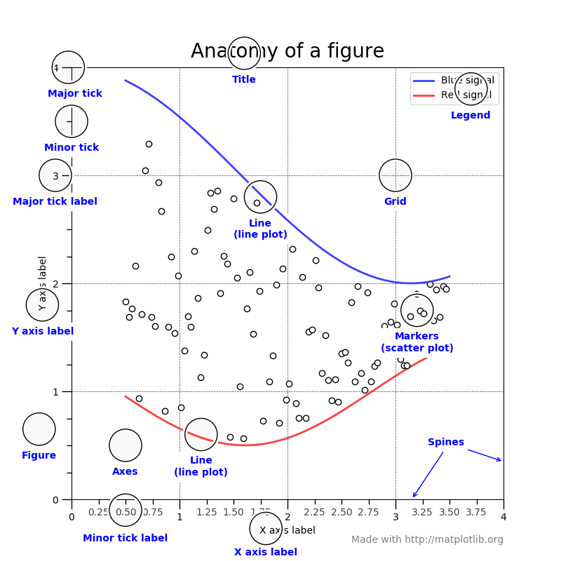
For consistent figure changes, define your own stylesheets that are basically a list of parameters to tune the aspect of the figure elements. See https://matplotlib.org/tutorials/introductory/customizing.html for more info.
We can also plot 2D data arrays.
noise = np.random.random((256,256))
plt.figure()
plt.imshow(noise)
<matplotlib.image.AxesImage at 0x7f39e2ef9438>

We can also add a colorbar and adjust the colormap.
plt.figure()
plt.imshow(noise, cmap=plt.cm.gray)
plt.colorbar()
<matplotlib.colorbar.Colorbar at 0x7f39e167e780>

Choose your colormaps wisely !
When doing such colorplots, it is easy to lose the interesting features by setting a colormap that is not adapted to the data.
Also, when producing scientific figures, think about how will your plot will look like to colorblind people or in greyscales (as it can happen in printed articles...).
See the interesting discussion on matplotlib website: https://matplotlib.org/users/colormaps.html.
Do it yourself:
With miscellaneous routines of scipy we can get an example image:
import scipy.misc
raccoon = np.array(scipy.misc.face())
Write a script to print shape and dtype the raccoon image. Next plot the image using matplotlib.
print("shape of raccoon = ", raccoon.shape)
print("dtype of raccoon = ", raccoon.dtype)
shape of raccoon =  (768, 1024, 3)
dtype of raccoon =  uint8
plt.imshow(raccoon)
<matplotlib.image.AxesImage at 0x7f39e00aba58>

Write a script to generate a border around the raccoon image (for example a 20 pixel size black border; black color code is 0 0 0)
Do it again without losing pixels and generate then a raccoon1 array/image
- Mask the face of the raccoon with a grey circle (centered of radius 240 at location 690 260 of the raccoon1 image; grey color code is for example (120 120 120)). Tip: check the np.indices function.
- Mask the face of the raccoon with a grey square by using NumPy broadcast capabilities (height and width 480 and same center as before)
We propose to smooth the image : the value of a pixel of the smoothed image is the the average of the values of its neighborhood (ie the 8 neighbors + itself).
Solution 0
Write a script to generate a border around the raccoon image (for example a 20 pixel size black border; black color code is 0 0 0)
raccoon[0:20, :, :] = 0
raccoon[-20:-1, :, :] = 0
raccoon[:, 0:20, :] = 0
raccoon[:, -20:-1, :] = 0
plt.imshow(raccoon)
<matplotlib.image.AxesImage at 0x7f39ce79dbe0>

Solution 1
Do it again without losing pixels and generate then a raccoon1 array/image
raccoon = np.array(scipy.misc.face())
print("shape of raccoon = ", raccoon.shape)
n0, n1, n2 = raccoon.shape
raccoon1 = np.zeros((n0+40, n1+40, n2), dtype = np.uint8)
raccoon1[20:20+n0, 20:20+n1, :] = raccoon[:,:,:]
print("shape of raccoon1 = ", raccoon1.shape)
plt.imshow(raccoon1)
shape of raccoon =  (768, 1024, 3)
shape of raccoon1 =  (808, 1064, 3)
<matplotlib.image.AxesImage at 0x7fee9e085a30>

Solution 2.A
Mask the face of the raccoon with a grey circle (centered of radius 240 at location 690 260 of the raccoon1 image; grey color code is for example (120 120 120))
raccoon2A = raccoon1.copy()
x_center = 260
y_center = 690
radius = 240
x_max, y_max, z = raccoon2A.shape
for i in range(x_max):
    for j in range(y_max):
        if ((j - y_center)**2 + (i-x_center)**2) <= radius**2:
            raccoon2A[i, j, :] = 120
plt.imshow(raccoon2A)
<matplotlib.image.AxesImage at 0x7fee97f77730>

Use the np.indices function:
- compute a matrix distances such that distances contains the distance to the center of the radius
- compute a boolean mask by applying a condition on the distances
- use the mask to set a gray value to the elements that fullfill the condition
racccoon3A = raccoon1.copy()
x_center = 260
y_center = 690
radius = 240
nb_lines, nb_cols,_  = raccoon3A.shape
X, Y = np.indices((nb_lines, nb_cols))
distances = np.sqrt((X-x_center)**2+(Y-y_center)**2)
mask = distances < radius
raccoon3A[mask] = 120
plt.imshow(raccoon3A)
<matplotlib.image.AxesImage at 0x7fee9c70eb20>

Solution 2.B
Mask the face of the raccoon with a grey square by using NumPy broadcast capabilities (height and width 480 and same center as before)
raccoon2B = raccoon1.copy()

raccoon2B[x_center-radius:x_center+radius, y_center-radius:y_center+radius, :] = 120

plt.imshow(raccoon2B)
<matplotlib.image.AxesImage at 0x7f39ce6410b8>

Solution 3
We propose to smooth the image : the value of a pixel of the smoothed image is the the average of the values of its neighborhood (ie the 8 neighbors + itself).
import scipy.misc
raccoon = scipy.misc.face().astype(np.uint16)
n0, n1, n2 = raccoon.shape
raccoon1 = np.zeros((n0, n1, n2), dtype = np.uint8)
for i in range(n0):
    for j in range(n1):
        if ((i!=0) and (i!=n0-1) and (j!=0) and (j!=n1-1)):
            tmp = (
                raccoon[i, j] + raccoon[i+1, j] + raccoon[i-1, j] + raccoon[i, j+1] + raccoon[i, j-1]
                + raccoon[i+1, j+1] + raccoon[i-1, j-1] + raccoon[i+1, j-1] + raccoon[i-1, j+1])
            raccoon1[i, j] = tmp/9
plt.imshow(raccoon1)
<matplotlib.image.AxesImage at 0x7f39ce629278>

Extra :
- Try to optimize (vectorization can be a solution)
- You can check what is a "sum area table" (or integral image) https://en.wikipedia.org/wiki/Summed-area_table and how to use it in our example.
- compute the area image (check the "cumsum" numpy function)
- use it to smooth your image.
Solution extra
def smooth(img):
    img = img.astype(np.uint16)
    n0, n1, n2 = img.shape
    img1 = np.zeros((n0, n1, n2), dtype=np.uint16)
    for i in range(n0):
        for j in range(n1):
            if ((i!=0) and (i!=n0-1) and (j!=0) and (j!=n1-1)):
                tmp = (
                    img[i, j] + img[i+1, j] + img[i-1, j] + img[i, j+1] + img[i, j-1] +
                    img[i+1, j+1] + img[i-1, j-1] + img[i+1, j-1] + img[i-1, j+1])
                img1[i, j] = tmp/9
    return img1.astype(np.uint8)


def smooth1(img):
    img = img.astype(np.uint16)
    n0, n1, n2 = img.shape
    img1 = np.zeros((n0, n1, n2), dtype=np.uint16)
    img1[1:n0-1, 1:n1-1] = (
        img[1:n0-1,1:n1-1] + img[2:n0, 1:n1-1] + img[0:n0-2, 1:n1-1] + img[1:n0-1, 2:n1] +
        img[1:n0-1, 0:n1-2] + img[2:n0, 2:n1] + img[0:n0-2, 0:n1-2] + img[2:n0, 0:n1-2] +
        img[0:n0-2, 2:n1])
    img1 = img1/9
    return img1.astype(np.uint8)


def smooth2(img):
    from scipy import signal
    img = img.astype(np.uint16)
    square8 = np.ones((3, 3), dtype=np.uint16)
    for i in range(3):
        img[:, :, i] = signal.fftconvolve(img[:, :, i], square8, mode='same')/9
    return img.astype(np.uint8)


def smooth3(img):
    from scipy import signal
    img = img.astype(np.uint16)
    n0, n1, n2 = img.shape
    img1 = np.zeros((n0, n1, n2), dtype=np.uint16)
    square8 = np.ones((3, 3), dtype=np.uint16)
    for i in range(3):
        img1[:, :, i] = signal.convolve2d(img[:, :, i], square8, mode='same')/9
    return img1.astype(np.uint8)


def smooth4(img):
    img = img.astype(np.uint16)
    n0, n1, n2 = img.shape
    img1 = np.zeros((n0, n1, n2), dtype=np.uint16)
    sum_area = np.cumsum(np.cumsum(img, axis=0), axis=1)
    img1[2:n0-1, 2:n1-1] = (
        sum_area[3:n0, 3:n1] + sum_area[0:n0-3, 0:n1-3] -
        sum_area[3:n0, 0:n1-3] - sum_area[0:n0-3, 3:n1])
    img1 = img1/9
    return img1.astype(np.uint8)


def smooth_loop(method, niter, img):
    for i in range(niter):
        img = method(img)
    return img

import scipy.misc
raccoon = scipy.misc.face()
%timeit smooth_loop(smooth, 1, raccoon)
%timeit smooth_loop(smooth1, 1, raccoon)
%timeit smooth_loop(smooth2, 1, raccoon)
%timeit smooth_loop(smooth3, 1, raccoon)
%timeit smooth_loop(smooth4, 1, raccoon)

raccoon = smooth_loop(smooth1, 20, raccoon)
plt.imshow(raccoon)
5.71 s ± 178 ms per loop (mean ± std. dev. of 7 runs, 1 loop each)
25.3 ms ± 96.6 µs per loop (mean ± std. dev. of 7 runs, 10 loops each)
233 ms ± 640 µs per loop (mean ± std. dev. of 7 runs, 1 loop each)
78.7 ms ± 442 µs per loop (mean ± std. dev. of 7 runs, 10 loops each)
106 ms ± 370 µs per loop (mean ± std. dev. of 7 runs, 10 loops each)
<matplotlib.image.AxesImage at 0x7f39c9a936d8>
