Advanced matplotlib
Pierre Augier (LEGI), Cyrille Bonamy (LEGI), Eric Maldonado (Irstea), Franck Thollard (ISTerre), Christophe Picard (LJK), Loïc Huder (ISTerre)
Introduction
This is the second part of the introductive presentation given in the Python initiation training.
The aim is to present more advanced usecases of matplotlib.
Quick reminders
import matplotlib.pyplot as plt
import numpy as np
X = np.arange(0, 2, 0.01)
Y = np.exp(X) - 1
plt.plot(X, X, linewidth=3)
plt.plot(X, Y)
plt.plot(X, X ** 2)
plt.xlabel("Abscisse")
plt.ylabel("Ordinate")
Text(0, 0.5, 'Ordinate')

Object-oriented plots
While doing the job, the previous example does not allow to unveil the power of matplotlib. For that, we need to keep in mind that in matplotlib plots, everything is an object.
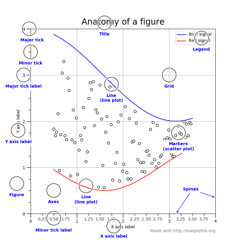
It is therefore possible to change any aspect of the figure by acting on the appropriate objects.
The same example with objects
fig = plt.figure()
print("Fig is an instance of", type(fig))
ax = fig.add_subplot(111) # More on subplots later...
print("Ax is an instance of", type(ax))
X = np.arange(0, 2, 0.01)
Y = np.exp(X) - 1
# Storing results of the plot
l1 = ax.plot(X, X, linewidth=3, label="Linear")
l2 = ax.plot(X, X ** 2, label="Square")
l3 = ax.plot(X, Y, label="$y = e^{x} - 1$")
xlab = ax.set_xlabel("Abscissa")
ylab = ax.set_ylabel("Ordinate")
ax.set_xlim(0, 2)
ax.legend()
Fig is an instance of <class 'matplotlib.figure.Figure'> Ax is an instance of <class 'matplotlib.axes._subplots.AxesSubplot'>
<matplotlib.legend.Legend at 0x7fee4c574dc0>

# ax.plot returns in fact a list of the lines plotted by the instruction
print(type(l3))
# In this case, we plotted the lines one by one so l3 contains only the line corresponding to the exp function
exp_line = l3[0]
print(type(exp_line))
<class 'list'> <class 'matplotlib.lines.Line2D'>
This way, we can have access to the Line2D objects and therefore to all their attributes (and change them!). This includes:
- get_data/set_data: to get/set the numerical xdata, ydata of the line
- get_color/set_color: to get/set the color of the line
- get_marker/set_marker: to get/set the markers
- ...
See https://matplotlib.org/api/_as_gen/matplotlib.lines.Line2D.html for the complete list.
Note: Line2D is based on the Artist class from which any graphical element inherits (lines, ticks, axes...).
from calendar import day_name
weekdays = list(day_name)
print(weekdays)
temperatures = [20.0, 22.0, 16.0, 18.0, 17.0, 19.0, 20.0]
fig, ax = plt.subplots()
ax.plot(temperatures, marker="o", markersize=10)
ax.set_xlabel("Weekday")
ax.set_ylabel("Temperature ($^{\circ}C$)")
['Monday', 'Tuesday', 'Wednesday', 'Thursday', 'Friday', 'Saturday', 'Sunday']
Text(0, 0.5, 'Temperature ($^{\\circ}C$)')

# Change locations
ax.set_yticks(np.arange(15, 25, 0.5))
# Change locations AND labels
ax.set_xticks(range(7))
ax.set_xticklabels(weekdays)
ax.set_xlabel("")
# Show the updated figure
fig

With Locators
Locators are objects that give rules to generate the tick locations. See https://matplotlib.org/api/ticker_api.html.

For example, for the yticks in the previous example, we could have done
import matplotlib.ticker as ticker
# Change locator for the major ticks of yaxis
ax.yaxis.set_major_locator(ticker.MultipleLocator(0.5))
fig
Major and minor ticks
matplotlib provides two types of ticks: major and minor. The parameters and aspect of the two kinds can be handled separately.
import matplotlib.ticker as ticker
# Change locator for the major ticks of yaxis
ax.yaxis.set_major_locator(ticker.MultipleLocator(1.0))
ax.yaxis.set_minor_locator(ticker.MultipleLocator(0.5))
fig

An application: subplots
fig, axes = plt.subplots(nrows=1, ncols=3, sharey=True)
"""
# Equivalent to
fig = plt.figure()
axes = []
axes.append(fig.add_subplot(131))
axes.append(fig.add_subplot(132, sharey=axes[0]))
axes.append(fig.add_subplot(133, sharey=axes[0]))
"""
# This is only to have the same colors as before
color_cycle = plt.rcParams["axes.prop_cycle"].by_key()["color"]
X = np.arange(0, 2, 0.01)
Y = np.exp(X) - 1
axes[0].set_title("Linear")
axes[0].plot(X, X, linewidth=3, color=color_cycle[0])
axes[1].set_title("Square")
axes[1].plot(X, X ** 2, label="Square", color=color_cycle[1])
axes[2].set_title("$y = e^{x} - 1$")
axes[2].plot(X, Y, label="$y = e^{x} - 1$", color=color_cycle[2])
axes[0].set_ylabel("Ordinate")
for ax in axes:
ax.set_xlabel("Abscissa")
ax.set_xlim(0, 2)

Fancier subplots with gridspec
import matplotlib.gridspec as gridspec
fig = plt.figure()
gs = gridspec.GridSpec(2, 2, figure=fig) # 2 rows and 2 columns
X = np.arange(-3, 3, 0.01) * np.pi
ax1 = fig.add_subplot(gs[0, 0]) # 1st row, 1st column
ax2 = fig.add_subplot(gs[1, 0]) # 2nd row, 1st column
ax3 = fig.add_subplot(gs[:, 1]) # all rows, 2nd column
ax1.plot(X, np.cos(2 * X), color="red")
ax2.plot(X, np.sin(2 * X), color="magenta")
ax3.plot(X, X ** 2)
[<matplotlib.lines.Line2D at 0x7fee4c22a0a0>]

Interactivity (https://matplotlib.org/users/event_handling.html)
Know first that other plotting libraries offers interactions more smoothly (plotly, bokeh, ...). Nevertheless, matplotlib gives access to backend-independent methods to add interactivity to plots.
These methods use Events to catch user interactions (mouse clicks, key presses, mouse hovers, etc...).
These events must be connected to callback functions using the mpl_connect method of Figure.Canvas:
fig = plt.figure()
fig.canvas.mpl_connect(self, event_name, callback_func)
The signature of callback_func is:
def callback_func(event)
where event is a matplotlib.backend_bases.Event. The following events are recognized
- 'button_press_event'
- 'button_release_event'
- 'draw_event'
- 'key_press_event'
- 'key_release_event'
- 'motion_notify_event'
- 'pick_event'
- 'resize_event'
- 'scroll_event'
- 'figure_enter_event',
- 'figure_leave_event',
- 'axes_enter_event',
- 'axes_leave_event'
- 'close_event'
N.B. : Figure.Canvas takes care of the rendering of the figure (independent of the used backend) which is why it is used to handle events.
A simple example: changing the color of a line
# Jupyter command to enable interactivity
%matplotlib notebook
f = plt.figure()
ax = f.add_subplot(111)
X = np.arange(0, 10, 0.01)
(l,) = plt.plot(X, X ** 2)
def change_color(event):
l.set_color("green")
f.canvas.mpl_connect("button_press_event", change_color)
9
Enhanced interactivity: a drawing tool
f2 = plt.figure()
ax2 = f2.add_subplot(111)
ax2.set_aspect("equal")
x_data = []
y_data = []
(l,) = ax2.plot(x_data, y_data, marker="o")
def add_datapoint(event):
x_data.append(event.xdata)
y_data.append(event.ydata)
l.set_data(x_data, y_data)
f2.canvas.mpl_connect("button_press_event", add_datapoint)
9
But, here we are referencing x_data and y_data in add_datapoint that are defined outside the function : this breaks encapsulation !
A nicer solution would be to use an object to handle the interactivity. We can also take advantage of this to add more functionality (such as clearing of the figure when the mouse exits) :
class InteractivePlot:
def __init__(self, figure):
self.ax = figure.add_subplot(111)
self.ax.set_aspect("equal")
self.x_data = []
self.y_data = []
(self.interactive_line,) = self.ax.plot(self.x_data, self.y_data, marker="o")
# Need to keep the callbacks references in memory to have the interactivity
self.button_callback = figure.canvas.mpl_connect(
"button_press_event", self.add_datapoint
)
self.clear_callback = figure.canvas.mpl_connect(
"figure_leave_event", self.clear
)
def add_datapoint(self, event):
if event.button == 1: # Left click
self.x_data.append(event.xdata)
self.y_data.append(event.ydata)
self.update_line()
elif event.button == 3: # Right click
self.x_data = []
self.y_data = []
(self.interactive_line,) = self.ax.plot(
self.x_data, self.y_data, marker="o"
)
def clear(self, event):
self.ax.clear()
self.x_data = []
self.y_data = []
(self.interactive_line,) = self.ax.plot(self.x_data, self.y_data, marker="o")
def update_line(self):
self.interactive_line.set_data(self.x_data, self.y_data)
f = plt.figure()
ip = InteractivePlot(f)
More examples could be shown but it always revolves around the same process: connecting an Event to a callback function.
Note that the connection can be severed using mpl_disconnect that takes the callback id in arg (in the previous case self.button_callback or self.clear_callback.
Some usages of interactivity:
- Print the value of a point on click
- Trigger a plot in the third dimension of a 3D plot displayed in 2D
- Save a figure on closing
- Ideas ?
Animations
From the matplotlib page (https://matplotlib.org/api/animation_api.html):
The easiest way to make a live animation in matplotlib is to use one of the Animation classes.
FuncAnimation Makes an animation by repeatedly calling a function func. ArtistAnimation Animation using a fixed set of Artist objects.
Example from matplotlib page
This example uses FuncAnimation to animate the plot of a sin function.
The animation consists in making repeated calls to the update function that adds at each frame a datapoint to the plot.
%matplotlib inline
from matplotlib import animation
fig, ax = plt.subplots()
xdata, ydata = [], []
(ln,) = plt.plot([], [], "ro")
def init():
ax.set_xlim(0, 2 * np.pi)
ax.set_ylim(-1, 1)
return (ln,)
def update(frame):
xdata.append(frame)
ydata.append(np.sin(frame))
ln.set_data(xdata, ydata)
return (ln,)
ani = animation.FuncAnimation(
fig, update, frames=np.linspace(0, 2 * np.pi, 128), init_func=init, blit=True
)
plt.show()

The previous code executed in a regular Python script should display the animation without problem. In a Jupyter Notebook, if we use %matplotlib inline, we can use IPython to display it in HTML.
from IPython.display import HTML
HTML(ani.to_jshtml())
Stroop test
The Stroop effect is when a psychological cause inteferes with the reaction time of a task.
A common demonstration of this effect (called a Stroop test) is naming the color in which a word is written if the word describes another color. This usually takes longer than for a word that is not a color.
Ex: Naming blue for
Funfact: As this test relies on the significance of the words, people that are more used to English should find the test more difficult !
In this part, we show how matplotlib animations can generate a Stroop test that shows random color words in random colors at random positions.
With FuncAnimation
We will generate a single object word whose position, color and text will be updated by the repeatedly called function.
import random
def generate_random_colored_word(words, colors):
displayed_text = random.choice(words).upper()
text_color = random.choice(colors)
xy_position = (random.random(), random.random())
return xy_position, displayed_text, text_color
def update(frame):
xy_position, displayed_text, text_color = generate_random_colored_word(
wordset, colorset
)
word.set_position(xy_position)
word.set_color(text_color)
word.set_text(displayed_text)
return word
fig, ax = plt.subplots()
colorset = ["red", "blue", "yellow", "green", "purple"]
wordset = colorset
xy_position, displayed_text, text_color = generate_random_colored_word(
wordset, colorset
)
word = ax.annotate(
displayed_text, xy_position, xycoords="axes fraction", color=text_color, size=36
)
ani = animation.FuncAnimation(fig, update, interval=1000)
plt.show()

from IPython.display import HTML
HTML(ani.to_jshtml())
With ArtistAnimation
Rather than updating through a function, ArtistAnimation requires to generate first all the Artists that will be displayed during the whole animation.
A list of Artists must therefore be supplied for each frame. Then, all frame lists must be compiled in a single list (of lists) that will be given in argument of ArtistAnimation.
In our case, to reproduce the behaviour above, we need to have only one word per frame. Each frame will therefore have a list of a single element (the colored word for this frame).
fig, ax = plt.subplots()
N_frames = 200
words = []
colorset = ["red", "blue", "yellow", "green", "purple"]
wordset = colorset
# Generate the list of lists of Artists.
for i in range(N_frames):
xy_position, displayed_text, text_color = generate_random_colored_word(
wordset, colorset
)
# The list of the frame contains only a single word
frame_artists = [
ax.annotate(
displayed_text,
xy_position,
xycoords="axes fraction",
color=text_color,
size=36,
)
]
words.append(frame_artists)
ani = animation.ArtistAnimation(fig, words, interval=1000)
plt.show()

from IPython.display import HTML
HTML(ani.to_jshtml())
Example with multiple Artists: two words at once from two wordsets !
# We can remove the axes for a cleaner test
fig = plt.figure()
ax = fig.add_subplot(111, frameon=False)
ax.set_xticks([])
ax.set_yticks([])
N_frames = 200
words = []
colorset = ["red", "blue", "yellow", "green", "purple"]
wordset = colorset
wordset2 = ["bed", "glue", "mellow", "grain", "people"]
# Generate the list of lists of Artists.
for i in range(N_frames):
xy_position, displayed_text, text_color = generate_random_colored_word(
wordset, colorset
)
xy_position2, displayed_text2, text_color2 = generate_random_colored_word(
wordset2, colorset
)
# The list of the frame contains only a single word
frame_artists = [
ax.annotate(
displayed_text,
xy_position,
xycoords="axes fraction",
color=text_color,
size=36,
),
ax.annotate(
displayed_text2,
xy_position2,
xycoords="axes fraction",
color=text_color2,
size=36,
),
]
words.append(frame_artists)
ani = animation.ArtistAnimation(fig, words, interval=1000)
plt.show()

from IPython.display import HTML
HTML(ani.to_jshtml())